Being home on a Sunday afternoon has many positive aspects, one of which a few days ago was to witness the sun’s rays floating into the rooms. After rather short and grey days of winter, the day I realise the sun is once again shining directly in my rooms, I am always very happy.

Every now and then I think about the times for sunrise and sundown, which I usually look up at the Austrian Institute for Meterology and Geodynamic (ZAMG) to see, how fast days are getting longer. I will use this opportunity to visualise the patterns of sunrise and sunset for my current hometown, which is Graz in the south of Austria.
Get the data
First, we need to load some packages. Since I want to scrape the times for sunrise and sunset from the page of ZAMG, we need to load rvest alongside the usual tidyverse.
library(rvest)
library(tidyverse)
library(lubridate)

theme_set(hrbrthemes::theme_ipsum(base_family = "Hind"))
Before we scrape, we need to check, whether we are allowed to, or not.
link <- "https://www.zamg.ac.at/cms/de/klima/klimauebersichten/ephemeriden/graz/?jahr=2018"

robotstxt::paths_allowed(link)## [1] TRUESeems to be OK.
After that, we go ahead to scrape the table of sunrise and sunset times. In order to find the appropriate tag for html_node(), I always use selectorgadget. Luckily the table is quite accessible, we simply need to select one node and extract the table. Since the column headings are duplicated and tibbles don’t like this, I set appropriate columns manually.
page <- read_html(link)

times <- page %>%
  html_node(".dynPageTable") %>%
  html_table() %>%
  set_names(c("day", "month", "year", "sunrise", "sunset",
              "moonrise", "moonset")) %>%
  as_tibble()
times
## # A tibble: 365 x 7
## day month year sunrise sunset moonrise moonset
## <dbl> <chr> <int> <chr> <chr> <chr> <chr>
## 1 1.00 Jänner 2018 07:44 16:19 16:01 06:37
## 2 2.00 Jänner 2018 07:44 16:20 17:06 07:43
## 3 3.00 Jänner 2018 07:44 16:21 18:18 08:39
## 4 4.00 Jänner 2018 07:44 16:22 19:33 09:27
## 5 5.00 Jänner 2018 07:44 16:23 20:48 10:05
## 6 6.00 Jänner 2018 07:44 16:25 22:00 10:38
## 7 7.00 Jänner 2018 07:44 16:26 23:10 11:08
## 8 8.00 Jänner 2018 07:43 16:27 ---- 11:35
## 9 9.00 Jänner 2018 07:43 16:28 00:16 12:00
## 10 10.0 Jänner 2018 07:43 16:29 01:21 12:26
## # ... with 355 more rowsThe table looks OK, but in order to do some plotting, we need to combine the information on day, month and year into one column.
sun_times <- times %>%
  mutate(date = paste(year, month, day, sep = "-") %>% ymd())
sun_times
## # A tibble: 365 x 8
## day month year sunrise sunset moonrise moonset date
## <dbl> <chr> <int> <chr> <chr> <chr> <chr> <date>
## 1 1.00 Jänner 2018 07:44 16:19 16:01 06:37 2018-01-01
## 2 2.00 Jänner 2018 07:44 16:20 17:06 07:43 2018-01-02
## 3 3.00 Jänner 2018 07:44 16:21 18:18 08:39 2018-01-03
## 4 4.00 Jänner 2018 07:44 16:22 19:33 09:27 2018-01-04
## 5 5.00 Jänner 2018 07:44 16:23 20:48 10:05 2018-01-05
## 6 6.00 Jänner 2018 07:44 16:25 22:00 10:38 2018-01-06
## 7 7.00 Jänner 2018 07:44 16:26 23:10 11:08 2018-01-07
## 8 8.00 Jänner 2018 07:43 16:27 ---- 11:35 2018-01-08
## 9 9.00 Jänner 2018 07:43 16:28 00:16 12:00 2018-01-09
## 10 10.0 Jänner 2018 07:43 16:29 01:21 12:26 2018-01-10
## # ... with 355 more rowsPlot the data
For this data I want to have the date from first of January to 31st of December on the x-axis, and the times of day when the sun rises and sets on the y-axis. For this, we need to gather our data, and then create a slightly hacky time variable. Since there is no class for time without date, I combine the information on sunset and sunrise times with today’s date.
gathered_times <- sun_times %>%
  gather(type, time, sunrise, sunset) %>%
  select(date, type, time) %>%
  mutate(time = paste0(today(), "-", time) %>% ymd_hm())
gathered_times## # A tibble: 730 x 3
## date type time
## <date> <chr> <dttm>
## 1 2018-01-01 sunrise 2018-02-13 07:44:00
## 2 2018-01-02 sunrise 2018-02-13 07:44:00
## 3 2018-01-03 sunrise 2018-02-13 07:44:00
## 4 2018-01-04 sunrise 2018-02-13 07:44:00
## 5 2018-01-05 sunrise 2018-02-13 07:44:00
## 6 2018-01-06 sunrise 2018-02-13 07:44:00
## 7 2018-01-07 sunrise 2018-02-13 07:44:00
## 8 2018-01-08 sunrise 2018-02-13 07:43:00
## 9 2018-01-09 sunrise 2018-02-13 07:43:00
## 10 2018-01-10 sunrise 2018-02-13 07:43:00
## # ... with 720 more rowsggplot(gathered_times, aes(date, time, colour = type)) +
geom_line() +
scale_y_datetime(date_breaks = "2 hours", date_labels = "%H:%M") +
labs(x = NULL, y = NULL, title = "Sunset and sunrise in Graz (Austria)")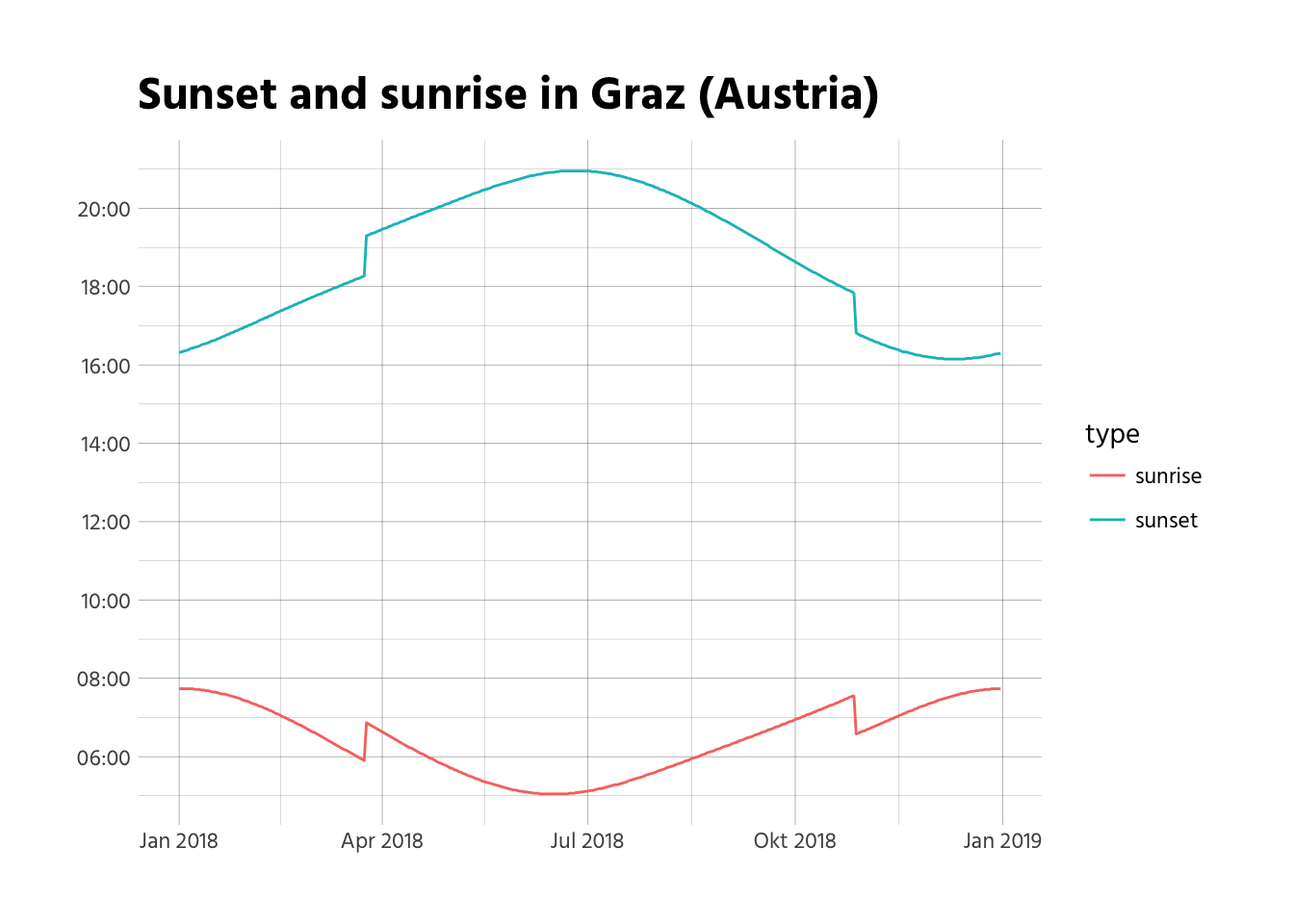 This already looks quite nice. We can clearly see the jumps in sunrise and sunset times that stem from daylight-saving.
For the final graph to look a bit prettier, I would like to add a few annotations:
- get rid of the legend and annotate inside the plot
- show a vertical line of today, with today’s length of day.
Let’s prepare those annotations:
labels <- tribble(~date,             ~type,     ~time,
                  ymd("2018-07-01"), "sunrise", ymd_hm("2018-02-13-07:00"),
                  ymd("2018-07-01"), "sunset",  ymd_hm("2018-02-13-19:00"))


# calculate todays length of day
day_length <- gathered_times %>%
  filter(date == today()) %>%
  spread(type, time) %>%
  mutate(day_length = sunset - sunrise) %>%
  pull(day_length) %>%
  round(2) %>%
  as.character()
And let’s plot the graph.
ggplot(gathered_times, aes(date, time, colour = type)) +
  geom_line(show.legend = F) +
  scale_y_datetime(date_breaks = "2 hours", date_labels = "%H:%M") +
  scale_color_brewer(palette = "Set1") +
  geom_vline(xintercept = today(), colour = "#4DAF4A") +
  geom_text(data = labels, aes(label = type), show.legend = F) +
  annotate("text", x = today() + 85, y = ymd_hm(paste(today(), "12:30", sep = "-")),
           label = paste0("Today's length of day: ", day_length, " hours."),
           colour = "#4DAF4A") +
  labs(x = NULL, y = NULL, title = "Sunset and sunrise in Graz (Austria)")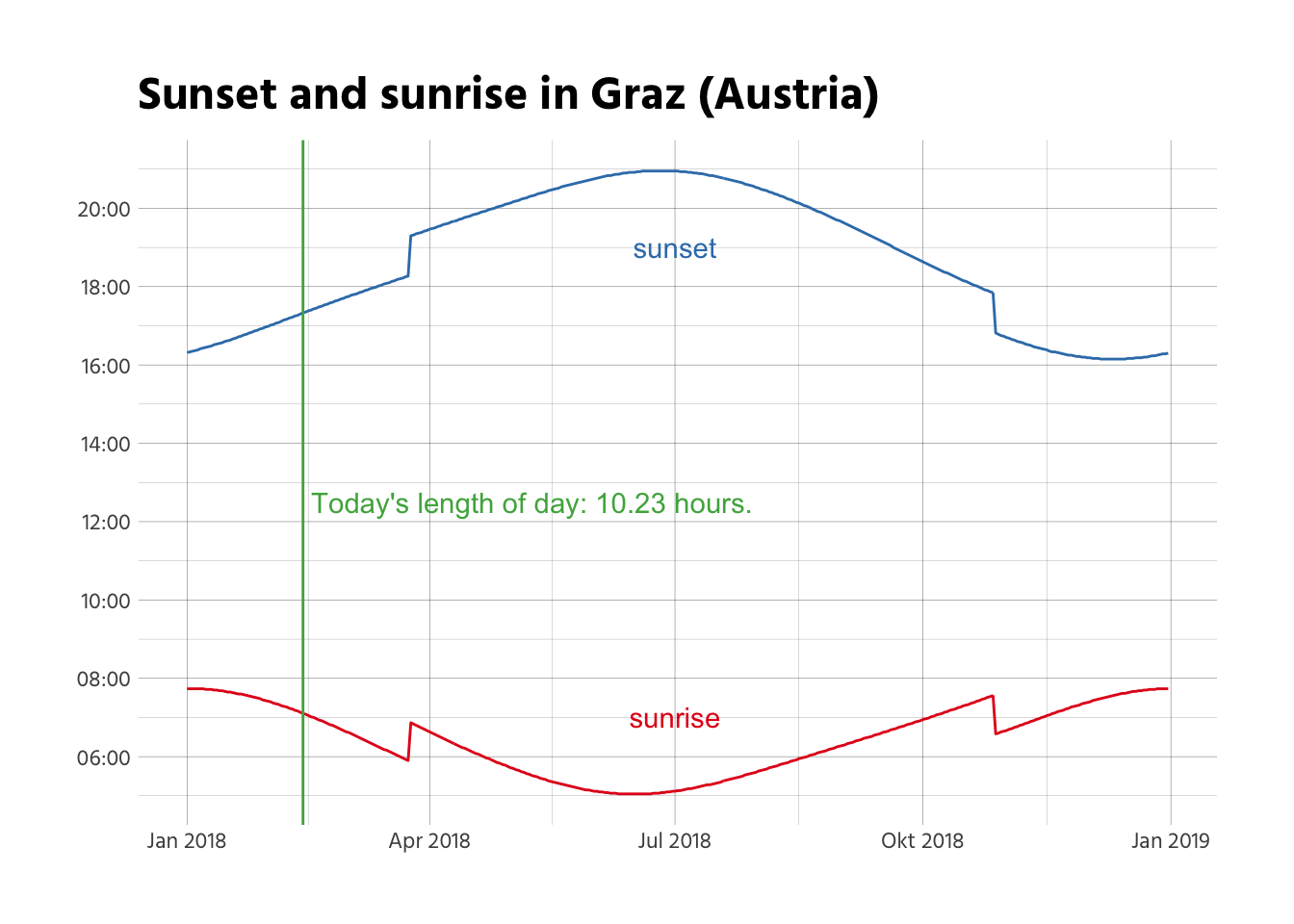
Ten hours and ~14 minutes (0.23 * 60 = 13.8) of possible daylight is not that much, but not bad either. In order to have better chances of having sunlight in my face, however, I should probably be getting up earlier, so I can walk back home from university before the sun has set. 🌅 Maybe this will finally change my habits for when to get up, although I doubt it a bit 🤷🏼♂️.